Before we get into the details of graphs, let's understand the real-life applications of graphs. Graphs exist everywhere, they are like a flow structure, that represents the pairwise relationship between objects.
They are basically used to represent a network - this network could refer to an intra-city network of roads or a connection network on social media.
What are Graphs
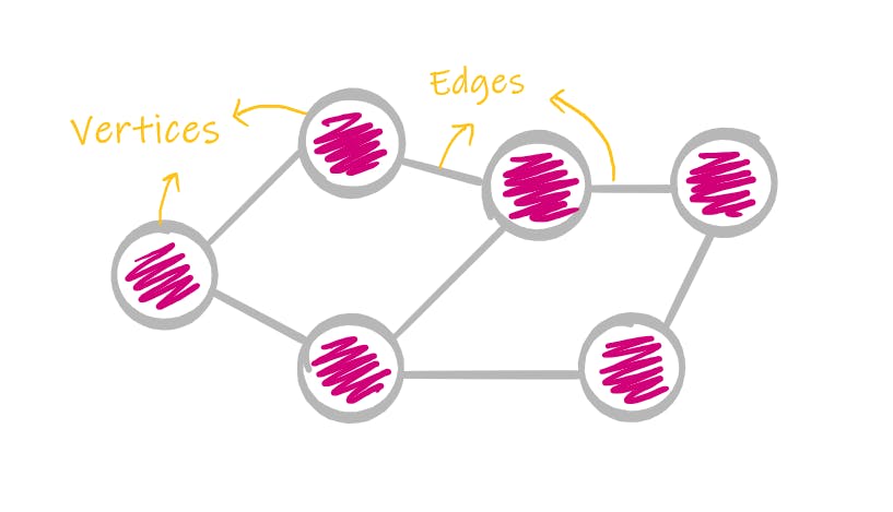
Graphs are data structures that constitute of 2 things - vertices and edges. Vertices are also known as nodes, and edges are also known as links or connections. Edges are what connect the nodes together.
Types of Edges
Edges can be of two types based on direction -
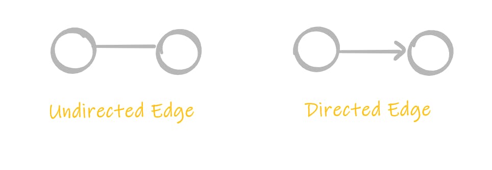
Undirected Edges: An undirected edge basically means a bidirectional edge, so if an edge connects A and B, it means A is connected to B, and B is connected to A.
Directed Edges: A directed edge has a single direction, and has a particular orientation. So A->B means A is connected to B but not vice versa.
Edges can be of two types based on weights-
Weighted Edge: If the edge/link carries some weight, it is known as a weighted edge. The weight refers to the cost it will take to travel through that edge, just like a tollway.
Unweighted Edge: If the edge/link does not carry any weight, it is known as an unweighted edge. It can be compared to a freeway, where it costs nothing to travel through that edge. Such edges are used to show if a connection exists or not.
Types of Graphs
Since we already know about the kind of edges, the types of graphs are easy to understand.
- Undirected graphs: A graph that consists of undirected edges is known as an undirected graph.
- Bidirectional graphs: A graph that consists of directed edges is known as a directed graph.
- Weighted graphs: A graph that consists of weighted edges is known as a weighted graph.
- Unweighted graphs: A graph that consists of unweighted edges is known as an unweighted graph.
Graph Representations
There exist 2 ways of representing a graph:
- Adjacency List
- Adjacency Matrix
Adjacency List
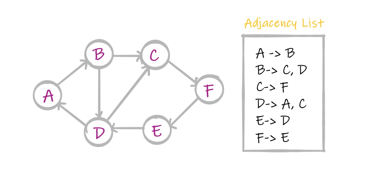
Adjacency list as the name suggests is a list of all the vertices, where each vertex stores all of its adjacent or neighboring vertices in the form of a list.
 #include<iostream >

#include < vector >

using namespace std;

vector < int > adj[10];

int main() {
  int x, y, nodes, edges;
  cin >> nodes;
  cin >> edges;
  for (int i = 0; i < edges; ++i) {
    cin >> x >> y;
    adj[x].push_back(y);
  }

  return 0;
}
- Space Complexity:
O(V+E) - Time Complexity to find if two nodes are connected to each other:
O(V)
The time complexity is of the worst-case scenario such as a complete graph, where every vertex is connected to each other.
Pros of Adjacency List:
- Complete graphs rarely exist in real life, hence the adjacency list is more efficient in terms of space.
Cons of Adjacency List:
- The access time to check whether an edge exists between 2 vertices is linear. This could be a huge disadvantage for the problems that require frequent lookups for edge connectivity.
Adjacency Matrix
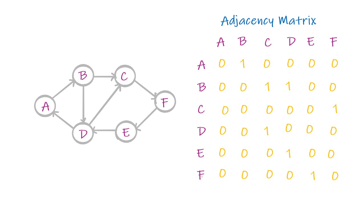
An adjacency matrix is a 2-dimensional matrix of dimensions V*V where V=vertices.
Each cell in the matrix, say graph[a][b] represents if vertex a is connected to b.
- For unweighted graphs, the value of a cell is either
1(connected)or0(not connected). - For weighted graphs, the value of a cell is either
0(not connected)orw(weight of the edge).
#include <iostream>

using namespace std;

int A[10][10];

int main() {
  int x, y, nodes, edges;
  cin >> nodes;
  cin >> edges;
  for (int i = 0; i < nodes; ++i) {
    for (int j = 0; j < nodes; ++j) {
      A[i][j] = 0;
    }
  }

  for (int i = 0; i < edges; ++i) {
    cin >> x >> y;
    A[x][y] = 1; //Mark the edges from vertex x to vertex y
  }
}
- Space Complexity: O(V*V)
- Time Complexity to find if two nodes are connected to each other: O(1)
Pros of Adjacency Matrix:
- Time Complexity to check if an edge exists between 2 vertices is O(1).
Cons of Adjacency Matrix:
- Can cause memory wastage, in the case of graphs where there are many vertices but few edges, since most of the cells would be filled by zero. Such graphs are known as Sparse Graphs.
Both of these representations have their own pros and cons and the decision to move forward with either of them depends upon the given problem and the given graph.
Graph Traversal Algorithms
Breadth First Search
To traverse a graph, you need to choose a vertex as a root/source/starting node. This vertex is from where we start our traversal.
BFS as the name stands means traversing a graph breadth by breadth. Breadth can also be thought of as a layer. We traverse the graph, layer by layer, or in a breadthwise manner.
For instance,
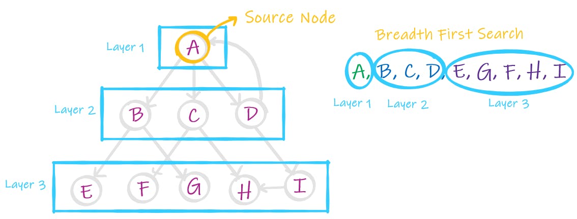
Now, a graph might contain a cycle, so we maintain a visited array to make sure we don't visit the same vertex again.
In simple words, this is what we do in BFS :
- We start from a vertex A, the source node, the node at Level 0.
- All the nodes directly connected to A, are at Level 1.
- Now you have a list of vertices at Level 1, we use them to find the vertices directly connected to them, the resulting vertices will be at Level 2.
- And we keep repeating this until we run out of the graph.
BFS implementation using Queue :
void BFS(int source) {
  // Mark all the vertices as not visited
  bool * visited = new bool[vertices];
  for (int i = 0; i < vertices; i++)
    visited[i] = false;

  // Create a queue for BFS
  queue < int > q;

  // Mark the current node as visited and push it in the queue
  visited[source] = true;
  q.push(source);

  // Eplore till we visit all the vertices
  while (!q.empty()) {
    // Pop a vertex from queue and print it
    int temp = q.front();
    cout << temp << " ";
    q.pop();

    // Get all adjacent vertices of the popped
    // vertex temp.
    // If a adjacent has not been visited,
    // then mark it visited and push it in the queue
    for (auto i = graph[temp].begin(); i != graph[temp].end(); ++i) {
      if (!visited[ * i]) {
        visited[ * i] = true;
        q.push( * i);
      }
    }
  }
}
- Space Complexity: O(B), for the queue where B is the maximum breadth/width of the graph.
- Time Complexity: O(V), where V=Vertices since we visit each vertex once.
Depth First Search
To traverse a graph, you need to choose a vertex as a root/source/starting node. This vertex is from where we start our traversal.
DFS as the name stands means traversing a graph in depth.
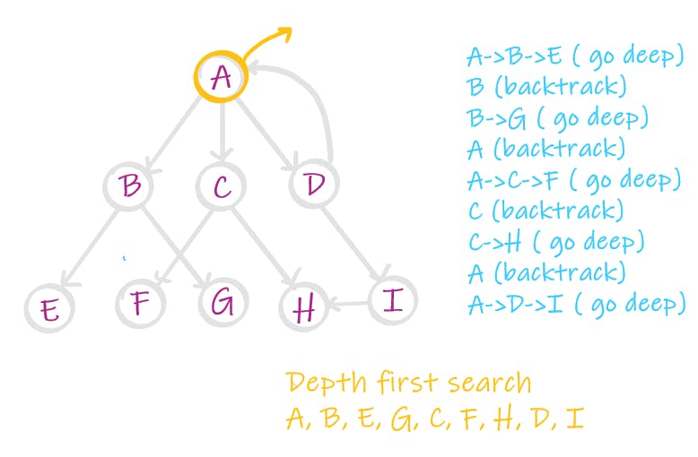
In DFS, we start from a source node, go deep as far as we can through a given path, and then backtrack to find an unexplored path, and then explore it in a depthwise fashion again. We keep doing this until the entire graph has been explored.
DFS implementation using Recursion:
void DFS(int sourceVertex, bool visited[]) {

  // mark the current source vertex as visited
  visited[sourceVertex] = true;
  cout << v << " ";

  // Recur for all the vertices adjacent to the current source vertex
  for (auto i = graph[sourceVertex].begin(); i != graph[sourceVertex].end(); ++i) {
    if (!visited[ * i]) {
      DFS( * i, visited);
    }
  }

}
- Space Complexity: O(D), for the recursion stack where D is the maximum depth of the graph.
- Time Complexity: O(V), where V=Vertices since we visit each vertex once.
Breadth-First Search can be implemented only using a queue, while Depth First Search can be implemented using Recursion or stack.
Do leave your feedback and suggestions :)
